Text classification using BERT
This example shows how to use a BERT model to classify documents. We use our usual Amazon review benchmark.
import torch
import torchtext
import random
import time
import sys
from collections import defaultdict
In this example, we'll use the Distilled BERT model, which is a bit faster than the other models. See the documentation of the transformers library for a list of the different pre-trained models. The example also works with the standard BERT. Other pre-trained models (XLNet, RoBERTa etc) might not work in this example because their tokenizers are more difficult to adapt to torchtext, but should work with small workarounds.
Each model released in the library comes with its own tokenizer, since they carry out the preprocessing in different ways and use different vocabularies, etc.
For the BERT model itself, we import the helper class that corresponds to our use case: in this case DistilBertForSequenceClassification. This uses an architecture suitable for classification tasks, with a linear output unit put on top of the highest Transformer layer in BERT. For other use cases, other helper classes are used.
from transformers import DistilBertTokenizer, DistilBertForSequenceClassification
model_name = 'distilbert-base-uncased'

#from transformers import BertTokenizer, BertForSequenceClassification
#model_name = 'bert-base-uncased'
The transformers library includes its own variant of the Adam optimizer, called AdamW. It's not strictly necessary to use it instead of PyTorch's standard Adam implementation, but I got slightly better accuracies with AdamW. Optionally, we also import WarmupLinearSchedule to reduce the learning rate gradually, but this didn't turn out to be useful when I tried it.
from transformers import AdamW, WarmupLinearSchedule
Quick side note about tokenization in BERT
BERT uses its own tokenization scheme, which is based on the WordPiece method (described in this paper, section 3). It uses a finite vocabulary, and when it encounters words outside the vocabulary, it will split them into pieces. This means that BERT will not run into out-of-vocabulary problems.
tokenizer = DistilBertTokenizer.from_pretrained(model_name)
To exemplify, if we consider a sentence with reasonably frequent words, BERT's tokenizer will separate the tokens but not split them. Note that this tokenizer will also put all strings in the lower case.
tokenizer.tokenize('Rolf lives in Gothenburg.')
If we tokenize a sentence including some less frequent words, each of these words will be split into two or more pieces. The pieces that were "chopped off" have the prefix ##.
tokenizer.tokenize('Margareta lives in Jonsered.')
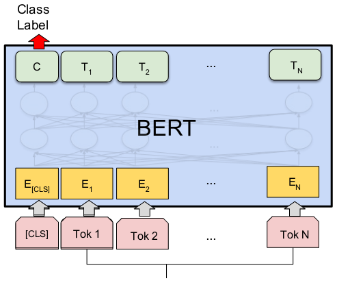
Before feeding a text into BERT, we will also add a special prefix token [CLS] and suffix token [SEP]. To compute the classification output, BERT will use the output at the [CLS] token.
tokenizer.tokenize('[CLS] This is a test. [SEP]')
Training the BERT model for our sentiment analysis task
We first do the preprocessing. Note that the evaluation function is slightly different since BERT computes the loss elsewhere, so we just return the number of correct guesses here.
def read_data(corpus_file, datafields, label_column, doc_start):
    with open(corpus_file, encoding='utf-8') as f:
        examples = []
        for line in f:
            columns = line.strip().split(maxsplit=doc_start)
            doc = columns[-1]
            label = columns[label_column]
            examples.append(torchtext.data.Example.fromlist([doc, label], datafields))
    return torchtext.data.Dataset(examples, datafields)

def evaluate_validation(scores, gold):
    guesses = scores.argmax(dim=1)
    return (guesses == gold).sum().item()
Now, let's implement the function that trains the BERT model for our classification task. The code is similar to our previous examples using CNNs, RNNs etc., and we'll comment just on the differences.
As in previous examples, we'll use torchtext to convert the texts into tensors. A little bit of work is needed here in order to make sure that torchtext and BERT use the same vocabularies.
BERT allows sequences of up to 512 tokens. Here, we'll use a shorter sequence length (128) in order to make training a bit faster and to save GPU memory. If you increase the sequence length, you may need to reduce the batch size in order not to run out of GPU memory.
The result will vary slight between runs, but typically we'll get an accuracy of about 0.88 with the distilled model and a maximum length of 128, which is better for this dataset than all models we have considered. If we increase the length or use a different model, the accuracy will increase a bit.
def main():

    MAX_LEN = 128

    # Create the tokenizer.
    tokenizer = DistilBertTokenizer.from_pretrained(model_name)
    #tokenizer = BertTokenizer.from_pretrained(model_name)

    # A small helper function that will call the BERT tokenizer and truncate.
    def bert_tokenize(sen):
        return tokenizer.tokenize(sen)[:MAX_LEN-2]

    # For preprocessing, we tell torchtext to use the tokenizer we defined above, and to automatically
    # add the [CLS] token in the beginning and [SEP] at the end, and that we use a dummy padding token
    # compatible with BERT.
    TEXT = torchtext.data.Field(sequential=True, tokenize=bert_tokenize, pad_token=tokenizer.pad_token,
                                init_token=tokenizer.cls_token, eos_token=tokenizer.sep_token)
    LABEL = torchtext.data.LabelField(is_target=True)
    datafields = [('text', TEXT), ('label', LABEL)]

    random.seed(0)

    print('Reading and tokenizing...')
    data = read_data('data/all_sentiment_shuffled.txt', datafields, label_column=1, doc_start=3)
    train, valid = data.split([0.8, 0.2])

    LABEL.build_vocab(train)
    TEXT.build_vocab(train)

    # Here, we tell torchtext to use the vocabulary of BERT's tokenizer.
    # .stoi is the map from strings to integers, and itos from integers to strings.
    TEXT.vocab.stoi = tokenizer.vocab
    TEXT.vocab.itos = list(tokenizer.vocab)

    device = 'cuda'

    # As mentioned above, you may need to reduce this in order to make it fit onto the GPU.
    # The BERT paper recommends a batch size of 16 or 32.
    batch_size = 32

    # Bucket iterators as in our previous RNN examples.
    train_iterator = torchtext.data.BucketIterator(
        train,
        device=device,
        batch_size=batch_size,
        sort_key=lambda x: len(x.text),
        repeat=False,
        train=True,
        sort=True)

    valid_iterator = torchtext.data.BucketIterator(
        valid,
        device=device,
        batch_size=batch_size,
        sort_key=lambda x: len(x.text),
        repeat=False,
        train=False,
        sort=True)

    # Let's load the pre-trained BERT model and put it onto the GPU. When using BERT for classification,
    # we need to tell it how many classes we'll use.
    print('Loading pre-trained BERT model...')
    n_classes = len(LABEL.vocab)
    model = DistilBertForSequenceClassification.from_pretrained(model_name, num_labels=n_classes)
    #model = BertForSequenceClassification.from_pretrained(model_name, num_labels=n_classes)
    model.cuda()


    #
    no_decay = ['bias', 'LayerNorm.weight']
    decay = 0.01
    optimizer_grouped_parameters = [
        {'params': [p for n, p in model.named_parameters() if not any(nd in n for nd in no_decay)], 'weight_decay': decay},
        {'params': [p for n, p in model.named_parameters() if any(nd in n for nd in no_decay)], 'weight_decay': 0.0}
    ]


    # As discussed above, we use the AdamW optimizer from the transformers library. It seems to
    # give slightly better results than the standard Adam.
    optimizer = AdamW(optimizer_grouped_parameters, lr=5e-5, eps=1e-8)
    #optimizer = torch.optim.Adam(optimizer_grouped_parameters, lr=5e-5)

    n_epochs = 4

    # I didn't see any improvements when trying to gradually reduce the learning rate, but
    # this might just need more careful tuning.
    #scheduler = WarmupLinearSchedule(optimizer, warmup_steps=0, t_total=len(train_iterator) // n_epochs)

    history = defaultdict(list)
    for i in range(n_epochs):

        t0 = time.time()

        loss_sum = 0
        n_batches = 0

        model.train()

        for batch in train_iterator:
            print('.', end='')
            sys.stdout.flush()

            # The tensor batch.text that comes from torchtext has the shape
            # (n_words, n_documents). BERT expects the opposite orientation,
            # so we transpose the tensor.
            text = batch.text.t()

            optimizer.zero_grad()

            # We apply the BERT model. Note that it computes the loss function, so
            # we won't have to compute the loss separately as in the previous examples.
            outputs = model(text, labels=batch.label)

            # The outputs tuple consists of the loss and the predictions. We'll just use the loss here.
            loss = outputs[0]

            loss.backward()
            optimizer.step()
            #scheduler.step()

            loss_sum += loss.item()
            n_batches += 1

            if n_batches % 50 == 0:
                print(f' ({loss_sum/n_batches:.4f})')

        train_loss = loss_sum / n_batches
        history['train_loss'].append(train_loss)

        print(f' ({train_loss:.4f})')

        n_correct = 0
        n_valid = len(valid)
        loss_sum = 0
        n_batches = 0

        model.eval()

        for batch in valid_iterator:
            print('.', end='')
            sys.stdout.flush()

            text = batch.text.t()

            with torch.no_grad():
                outputs = model(text, labels=batch.label)
                loss_batch, scores = outputs

            loss_sum += loss_batch.item()
            n_correct += evaluate_validation(scores, batch.label)
            n_batches += 1

            if n_batches % 50 == 0:
                print()

        val_acc = n_correct / n_valid
        val_loss = loss_sum / n_batches

        history['val_loss'].append(val_loss)
        history['val_acc'].append(val_acc)

        t1 = time.time()
        print()
        print(f'Epoch {i+1}: train loss = {train_loss:.4f}, val loss = {val_loss:.4f}, val acc: {val_acc:.4f}, time = {t1-t0:.4f}')

main()